Analytical Model
Analytical Model of Financial Market
Warning! Reading of the subsequent text assumes basic knowledge of probability theory.
The Analytical Model of Financial Market (or simply Analytical Model), utilized in SmartFolio, is based on Multidimensional Geometric Brownian Motion – the most common class of stochastic processes used in mathematical finance to model the dynamics of prices.
Consider  risky assets risky assets  available for the investments. Assume also that the investor has access to some riskless asset available for the investments. Assume also that the investor has access to some riskless asset  , which yields continuously compounded rate of return , which yields continuously compounded rate of return  that will be referred to as the riskless rate or risk-free rate. An investor expresses prices of assets that will be referred to as the riskless rate or risk-free rate. An investor expresses prices of assets  in units of asset . in units of asset .
Discounted price of asset  at time at time  is denoted by is denoted by  . Upper asterisk . Upper asterisk  in consequent text denotes transposition operation. in consequent text denotes transposition operation.
The main assumption of analytical model is given by the following system of stochastic differential equations, which describe evolution of discounted prices of assets :
In the above expression drift vector  (further referred to as the Mu vector), the vector of (further referred to as the Mu vector), the vector of
continuously compounded dividend yields  and volatility matrix and volatility matrix  consist of constant values, while elements of consist of constant values, while elements of  represent independent Wiener processes. represent independent Wiener processes.
Definition. For the sake of convenience the vector  , will be further referred to as the Excess Mu vector. , will be further referred to as the Excess Mu vector.
Definition. Matrix  is called Covariance Matrix. is called Covariance Matrix.
Note. Readers, who are not familiar with stochastic differential equations in continuous time, may interpret
 as very short time range, as very short time range,  as simple return in as simple return in  -th asset over -th asset over  and and  as as
normally distributed random vector, whose elements are independent of each other (and of components of
other vectors  ), have zero mean and variance . ), have zero mean and variance .
Denote by  diagonal matrix with elements of vector diagonal matrix with elements of vector  at the main diagonal. At the same time for diagonal matrix at the main diagonal. At the same time for diagonal matrix  denote column vector denote column vector  , whose elements are equal to diagonal elements of . , whose elements are equal to diagonal elements of .
In these notations the above system of stochastic differential equations reduces to:

A simple solution is presented below:
where components of the volatility vector  are calculated by means of the formula are calculated by means of the formula 
Using compact notation, this solution is written as
Definition. Components of vector
are called Expected Excess Growth Rates.
The above definition arises from the fact that for any 
where symbol  denotes mathematical expectation. denotes mathematical expectation.
On the other hand, it can be shown that
Note. Elements of  are also called Expected Instantaneous Rates of Return, reflecting the notion of expected simple rate of return over an infinitesimally short period of time. Indeed, it is easy to check that for are also called Expected Instantaneous Rates of Return, reflecting the notion of expected simple rate of return over an infinitesimally short period of time. Indeed, it is easy to check that for
any the following chain of equalities holds: 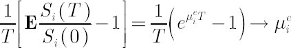 when when  approaches zero. approaches zero.
| |
|
 SiteMap\
 Contact Us
 The Theory
\
Details
\
analytical model
The Theory
\
Details
\
analytical model