![]()
Portfolio optimization results in the portfolio which is optimal respective to the selected optimality criterion and which satisfies the imposed portfolio constraints.
Excel Solver
IPOPT is significantly faster and more stable than Excel Solver, especially for middle- to large-size portfolios, but it is available in Professional Edition only.
Maximization of an expected constant relative risk aversion utility Class of utility functions which is exhausted by Logarithmic and Power utility functions. These utility functions are characterized by risk bearing proportional to wealth.. Maximization of portfolio expected excess growth rate Expected instantaneous rate of return (including Dividend yield) over the risk-free rate. as a special case.
Minimization of target shortfall probability [Stutzer; 2003]
Benchmark tracking
The first two criteria utilize, as an option, the so-called worst-case scenario optimization, which accounts for uncertainty in estimations of average returns [Garlappi, Uppal, Wang; 2005].
Optimization criteria details...
Walk-forward optimization makes it possible to verify whether theoretically optimal portfolios have any value in practice. There are two reasons why this might not be the case:
Portfolio optimization may result in overfitting the data, especially when performing optimization on relatively short time intervals and/or with too many portfolio components;
Historical data might be subject to pronounced non-stationarity.
The algorithm is extremely intuitive:
You select the lengths of in-sample and out-of-sample periods;
At each optimization
round in-sample and out-of-sample intervals are shifted forward by the
length of the out-of-sample period as shown in the picture below: 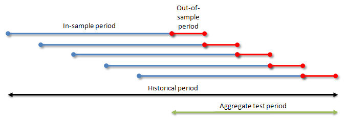
At each stage portfolio optimization is performed based on the data from the corresponding in-sample period. The results are then calculated by applying the obtained optimal weights to the corresponding out-of-sample period.
Lower and upper bounds on individual asset weights
Lower and upper bounds on asset groups
Short-selling constraint
Margin constraint Maximal leverage allowable in the asset. If the given asset admits trading on margin, which is equal to 20% of trade volume, then the corresponding margin constraint is equal to 5. Margin constraint for those assets that are not traded on margin is equal to 1. The fact that margin requirements must be satisfied simultaneously for all portfolio components, is expressed in the form of the aggregate margin constraint, that depends on all portfolio weights.
Zero weight in a riskless asset Other notations are Risk-free asset or Numeraire. It is the asset, in units of which portfolio wealth is measured. As a rule, the investor is nearly indifferent to changes in value of the riskless asset.
Zero weight in factors An asset which plays the role of an independent variable in the context of Factor-based asset pricing models.
Lower bound for expected excess growth rate
Upper bound for portfolio volatility The most common measure of risk. Defined as annualized standard deviation of returns.
Upper bound for portfolio normalized semi-volatility Equal to doubled Semi-volatility. Under the assumption of independent normally distributed logarithmic returns it coincides with Volatility. (for the historical portfolio only)
Upper bound for portfolio beta Measure of portfolio sensitivity to changes in price of the only Factor. Under the CAPM assumptions portfolio beta is calculated as the sum of products of individual betas and the corresponding portfolio weights. (for the analytical portfolio and one portfolio factor only)